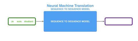
Hi! My name is Joshua Pritz. I’m a rising senior studying physics and math at Northwestern University. This summer, I am working with Dr. Marta Garcia Martinez in the Computational Science Division at Argonne National Lab. Our research concerns the application of Neural Network based approaches to the semantic segmentation of images detailing the feline spinal cord. This, too, is part of a larger effort to accurately map and reconstruct the feline spinal cord with respect to its relevant features – namely, neurons and blood vessels.
Prior to outlining my contribution to this work, it’s worth introducing the terminology used above and, thereafter, illustrating why it fits the motivations of our project. Image segmentation, generally, is the process of identifying an image’s relevant features by distinguishing its regions into different classes. In the case of our cat spine dataset, we are currently concerned with two classes: somas, the bodies of neurons in the spine, and background, everything else. Segmentation can be done by hand. Yet, with over 1800 images collected via x-ray tomography at Argonne’s Advanced Photon Source, this task is all but intractable. Given the homogeneity of features within our images, best exemplified by the similarity of blood vessels and somas (indicated in Figure 1 by a blue and red arrow, respectively), traditional computer segmentation techniques like thresholding and K-means clustering, which excel at identifying objects by contrast, would also falter in differentiating these features.
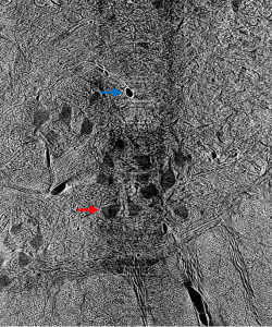
Figure 1: Contrast adjusted image of spinal cord. Blue arrow indicates blood vessel, while red arrow indicates soma.
Enter the Convolutional Neural Network (CNN), through which we perform what is known as semantic segmentation. Herein, a class label is associated with every pixel of an image. A CNN begins by assigning a trainable parameter, a weight, to each pixel in an incoming image. Then, in a step known as a convolution, it performs an affine operation on each submatrix of pixels in the image using a fixed scaling matrix called the kernel, which is then translated using another set of trainable parameters called biases. Convolutions create a rich feature map that can help to identify edges, areas of high contrast, and other features depending on the kernel used. Such operations also reduce the number of trainable parameters in succeeding steps, which is particularly helpful for large input images that necessarily subtend hundreds of thousands of weights and biases. Through activation functions that follow each convolution, the network then decides whether or not objects in the resultant feature map correspond to distinct classes.
This seems like a complicated way to perform an intuitive process, surely, but it begs a number of simple questions. How does the network know whether or not an object is in the class of interest? How can it know what to look for? Neural networks in all applications need to be trained extensively before they can perform to any degree of satisfaction. In the training process, a raw image is passed through the CNN. Its result – a matrix of ones and zeros corresponding respectively to our two classes of interest – is then compared to the image’s ground truth, a segmentation done by hand that depicts the desired output. In this comparison, the network computes a loss function and adjusts its weights and biases to minimize loss throughout training, similar to the procedure of least-squares regression. It takes time, of course, to create these ground truths necessary for training the CNN, but given the relatively small number of images needed for this repeatable process, the manual labor required pales in comparison to that of segmentation entirely by hand.
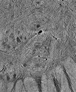
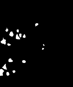
Figure 2: Cat spine image and its ground truth.
The question then becomes, and that which is of primary concern in this research, how can training, and the resulting performance of the CNN, be optimized given a fixed amount of training data? This question lives in a particularly broad parameter-space. First, there are a large number of tunable network criteria, known as hyperparameters (so as not to be confused with the parameters that underlie the action of the CNN), that govern the NN’s performance. Notably, these include epochs, one full pass of the training data through the network; batch-size, the number of images seen before parameters are updated; and learning rate, the relative amount parameters are updated after each training operation. For our network to perform exceptionally, we need to include enough epochs to reach convergence (the best possible training outcome) and tune the learning rate so as to meet it within a reasonable amount of time, while not allowing our network to diverge to a poor result (Bishop).
Second, we can vary the size of images in our training set, as well as the number of them. Smaller images, which are randomly cropped from our full-sized dataset, require a fewer number of trainable weights and biases, thus exhibiting quicker convergence. Yet, such images can neglect the global characteristics of certain classes, resulting in poorer performance on full-sized images. In choosing a number of images for our training set, we need balance whether or not enough data is present to affect meaningful training with oversampling of training data. To conclusively answer our project’s primary question without attempting to address the full breadth of the aforementioned parameter space, we developed the following systematic approach.
Prior to our efforts in optimization, we added notable functionality to our initial NN training script, which was written by Bo Lei of Carnegie Mellon University for the segmentation of materials science images and, herein, adapted to perform on our cat spine dataset. It employs the PyTorch module for open-source accessibility and uses the SegNet CNN architecture, which is noteworthy for its rendering of dense and accurate semantic segmentation outputs (Badrinarayanan, Kendall and Cippola). The first aspect of our adaptation of this script that required attention was its performance on imbalanced datasets. This refers to the dominance of one class, namely background, over a primary class of interest, the somas. To illustrate, an image constituted by 95 percent background and five percent soma could be segmented with 95 percent accuracy, a relatively high metric, by a network that doesn’t identify any somas. The result is a network that performs deceptively well, but yields useless segmentations. To combat this, our additional functionality determines the proportion made up by each class across an entire dataset, and scales the loss criterion corresponding to that class by the inverse of this proportion. Hence, loss corresponding to somas is weighted more highly, creating networks that prioritize their identification.
We also include data augmentation capabilities. At the end of each training epoch, our augmentation function randomly applies a horizontal or vertical flip to each image, as well as random rotations, with fifty percent probability. These transformed images, although derived from the same dataset, activate new weights and biases, thereby increasing the robustness of our training data. Lastly, we added visualization functionality to our script, which plots a number of metrics computed during training with respect to epoch. These metrics most notably include accuracy, the number of pixels segmented correctly divided by the total number of pixels, and the intersection-over-union score for the soma class, the number of correctly segmented soma pixels divided by the sum of those correctly identified with the class’s false positive and negatives (Jordan). We discuss the respective significance of these metrics insofar as evaluating a segmentation below.
Table 1: Hyperparameters used in training.
After including such functionalities our interest turned to optimizing the network’s hyperparameters as well as the computational time needed for training. To address the former, we first trained networks using our most memory-intensive dataset to determine an upper bound on the number of epochs needed to reach convergence in all cases. For the latter, we conducted equivalent training runs on the Cooley and Bebop supercomputing platforms. We found that Bebop offered an approximately two-fold decrease in training time per epoch, and conducted all further training runs on this platform. The remainder of the hyperparameters, with the exception of learning rate, are adapted from Stan et al. who perform semantic segmentation on similar datasets in MATLAB. Our preferred learning rate in this case was determined graphically, whereby we found that a rate of 10-4 did not permit effective learning during training on large images, while a rate of 10-2 led to large, chaotic jumps in our training metrics.
Table 2: List of tested cases depicting image size and number of images in training set.
Using such hyperparameters, listed in Table 1, for all successive training, we finally turned our attention to optimizing our networks’ performance with respect to the size of training images as well as the number of them used. Our initial training images (2300 by 1920 pixels) are very large compared to the size of images typically employed in NN training, which are in the ballpark of 224 by 224 pixels. Likewise, Stan et al. find that, despite training NNs to segment larger images, performance is optimal when using 1000 images of size 224 by 224 pixels. To see if this finding holds for our dataset, we developed ten cases that employ square images (with the exception of full-sized images) whose size and number are highlighted in Table 2. Image size varies from 100 pixels to 800 pixels per side, including training conducted on full-sized images, while image number varies from 250 to 2000. In this phase, one NN was trained and evaluated for each case.
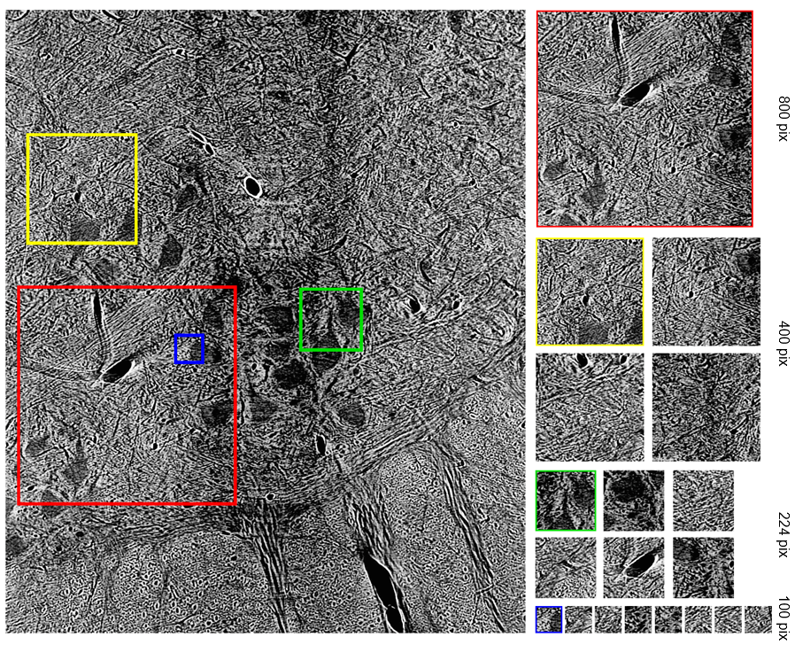
Figure 3: Detail of how smaller images were randomly cropped from full-sized image.
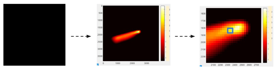
To standardize the evaluation of these networks, we applied each trained NN to two x-ray tomography test images. Compared to the 20+ minutes needed to segment one such image by hand, segmentation of one such 2300 by 1920 pixel image took averagely 12.03 seconds. Resulting from each network, we recorded the global accuracy, soma intersection-over-union (IoU) score, and boundary F-1 score corresponding to each segmentation. Accuracy is often high for datasets whose images are dominated by background, such is the case here, and rarely indicates the strength of performance on a class of interest. Soma IoU, on the other hand, is not sensitive to the imbalance in classes exhibited by our dataset. The boundary F-1 (BF1) score for each image is related to how close the boundary of somas in our NN segmentation is to that of the ground truth. Herein, we use a threshold of 2 pixels, so that if the boundary in our NN’s prediction remains within 2 pixels of the actual soma boundary, the segmentation would receive a 100% BF1 score (Fernandez-Moral, Martins and Wolf). Together with the soma IoU, these metrics provide a far more representative measurement of the efficacy of our network than solely global accuracy. For each network, we exhibit the average of these metrics over both test images in the table below, in addition to heatmaps for soma IoU and BF1 scores.
Figure 4: Heatmaps for BF1 and Soma IoU score for each case.
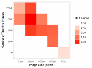
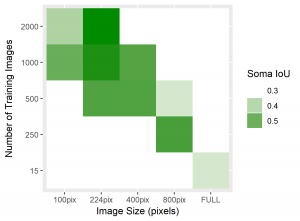
Table 3: Results from test image segmentations.
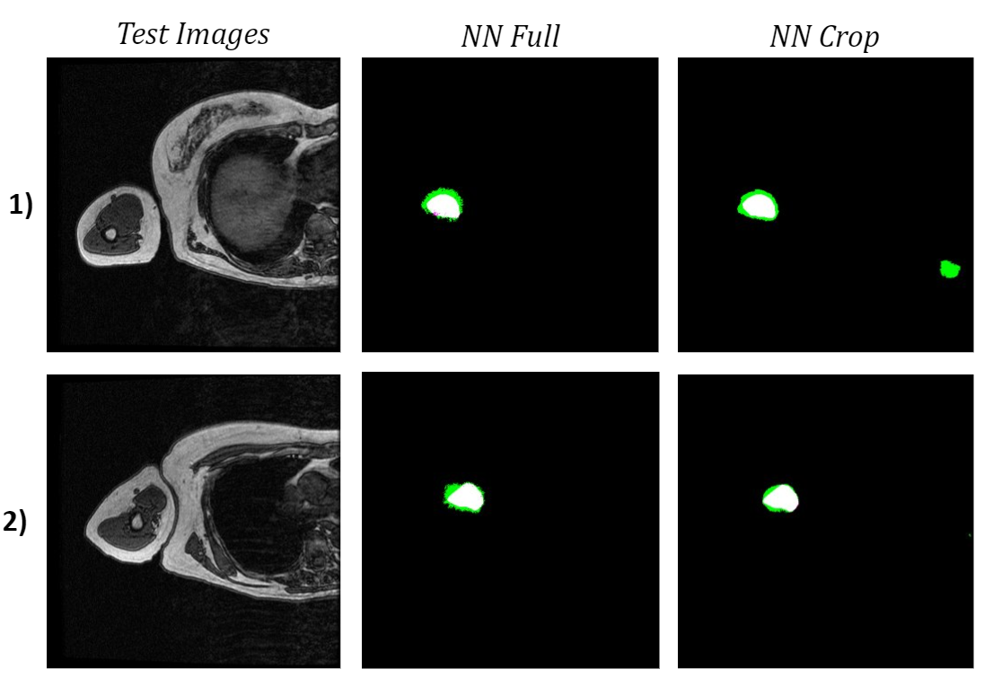
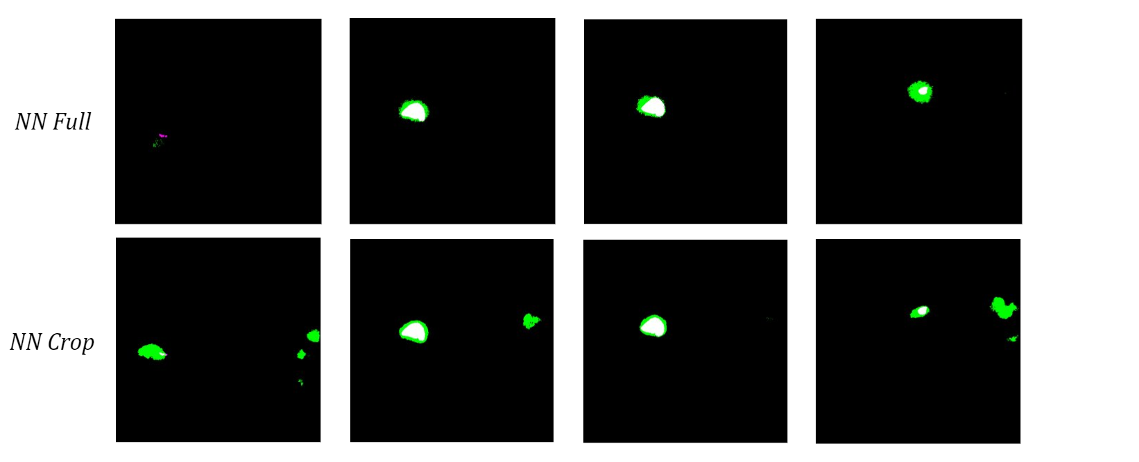
To visually inspect the quality of our NNs’ output, we overlay the predictions given by each network with the ground truth for the corresponding test image using a MATLAB script developed by Stan et al. This process indicates correctly identified soma pixels (true positives) in white and correctly identified background pixels in black (true negatives). Pink pixels, however, indicate those falsely identified as background (false negatives), while green pixels are misclassified as somas (false positives). We exhibit overlays resulting from a poorly performing network as well as those from our best performing network below.
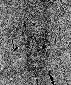
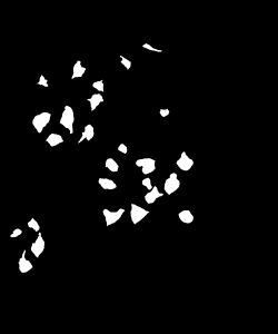
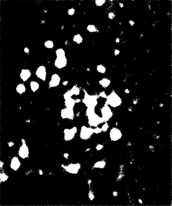

Figure 5: Top: raw test image (left) and test image ground truth (right). Bottom: NN (poorly performing) prediction (left) and overlay of prediction with ground truth (right).
The heatmaps above detailing soma IoU and BF1 scores visually represent trends in network performance with respect to image size and number. We recognize the following. The boundary F-1 score generally decreases when increasing the number of images in the training set. This is most likely due to oversampling in training data, by which resultant networks become too adept in performing on their training data and lose transferability that allows them to adapt to the novel test images. We recognize a similar trend in soma IoU. More so, network performance is seen to appreciate as we decrease the size of training images, until it reaches a maximum in the regime of 224 by 224 pixel images. The decrease in performance of networks trained on larger images may be explained by the lack of unique data. Despite a comparable number of training images, datasets of a larger image size are likely to have sampled the same portion of the original training images multiple times, resulting in redundant and ineffective training. The 100 by 100 pixel training images, on the other hand, are likely too small to capture the global character of somas in a single image given that some such features often approach 100 by 100 pixels in size. Hence, larger images may be needed to capture these essential morphological features. We find that highest performing network is that which was trained using 1000 images of size 224 by 224 pixels, exhibiting a global accuracy of 98.1%, a soma IoU of 68.6%, and a BF1 score of 31.0%. The overlay corresponding to this network shown in Figure 6 depicts few green and pink pixels, indicating an accurate segmentation.
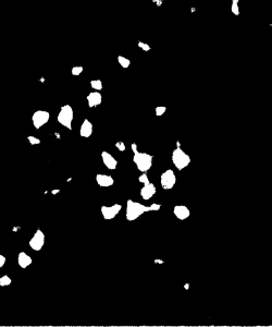
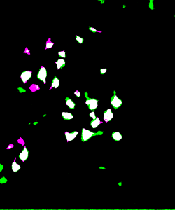
Figure 6: Top: raw test image (left) and test image ground truth (right). Bottom: NN (224pix1000num – best performing) prediction (left) and overlay of prediction with ground truth (right)
Ultimately, this work has shown that convolutional neural networks can be trained to distinguish classes from large and complex images. NN based approaches, too, provide an accurate and far quicker alternative to manual image segmentation and past computer vision techniques, given an appropriately trained network. Our optimization with respect to the size and number of images used for training has confirmed the findings of Stan et al. in showing that networks trained using a larger amount of smaller images perform better than those trained using full-sized images. Namely, our results indicate that 224 by 224 pixel images yield the highest performance with respect to accuracy, IoU, and BF1 scores. In the future, this work may culminate in the application of our best NN to the totality of the feline spinal cord dataset. With appropriate cleaning and parsing of the resultant segmentations, such a network could aid in novel 3D reconstructions of neuronal paths in the feline spinal cord.
References
Badrinarayanan, Vijay, Alex Kendall and Roberto Cipolla. “SegNet: A Deep Convolutional Encoder-Decoder Architecture for Image Segmentation.” IEEE Transactions on Patter Analysis and Machine Intelligence (2017): 2481-2495. Print.
Bishop, Christopher M. Pattern Recognition and Machine Learning. Cambridge: Springer, 2006. Print.
Fernandez-Moral, Eduardo, et al. “A New Metric for Evaluating Semantic Segmentation: Leveraging Global and Contour Accuracy.” 2018 IEEE Intelligent Vehicles Symposium (IV) (2018): 1051-1056. Print.
Jordan, Jeremy. “Evaluating Image Segmentation Models.” Jeremy Jordan, 18 Dec. 2018, www.jeremyjordan.me/evaluating-image-segmentation-models/. Website.
Stan, Tiberiu, et al. Optimizing Convolutional Neural Networks to Perform Semantic Segmentation on Large Materials Imaging Datasets: X-Ray Tomography and Serial Sectioning. Northwestern University, 19 June 2019. Print.
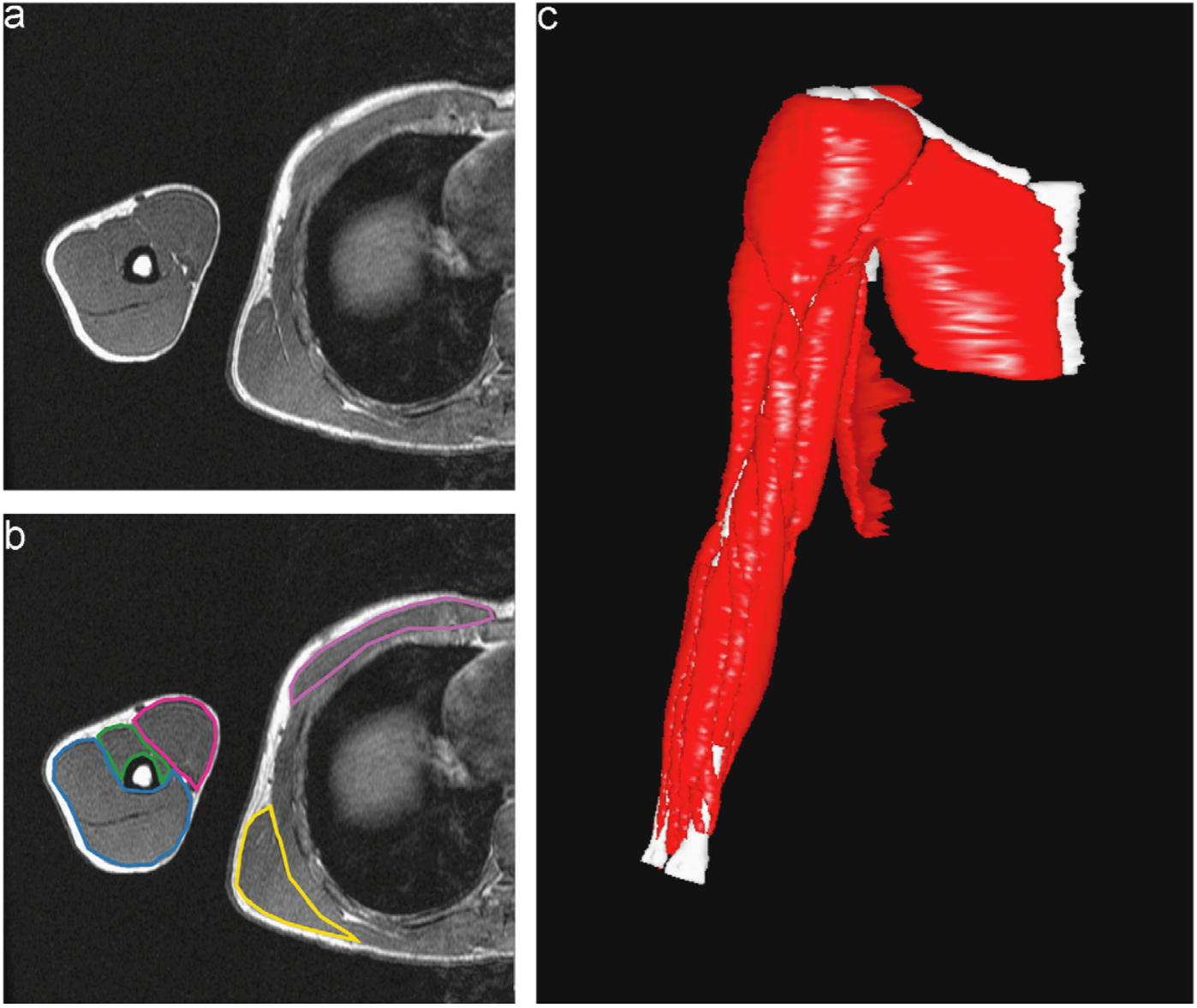
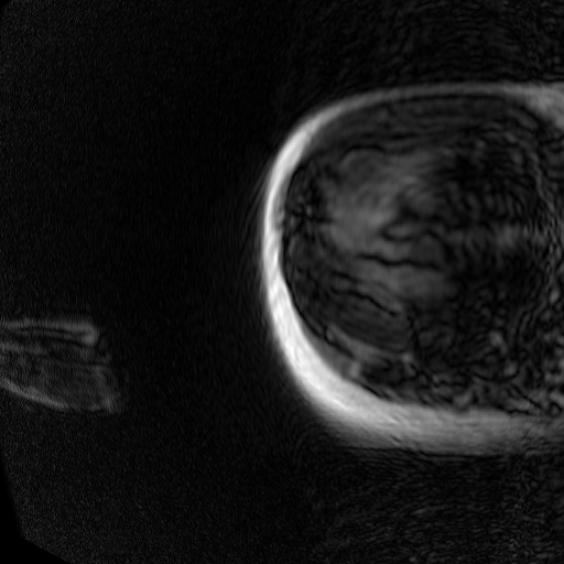
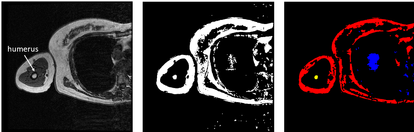 Figure 3: Original Image (left). Light Features as One Object (middle). Three Connected Components (right).
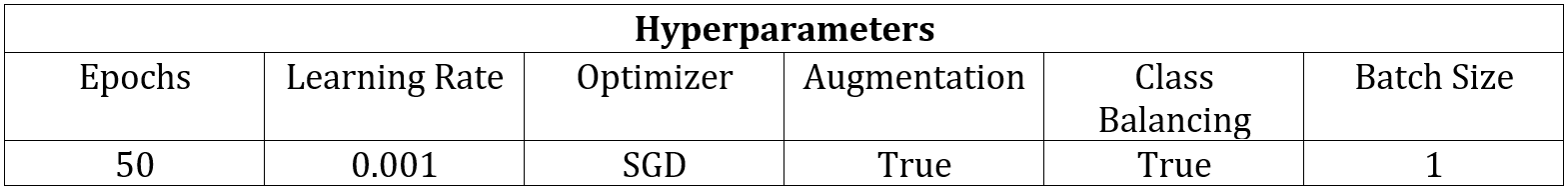 Table 1: Network Hyperparameters.
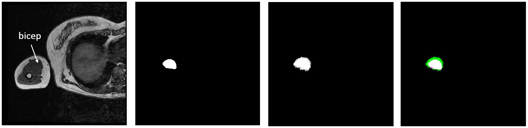 Figure 4: Test Image 1 (far left). Ground Truth Label (middle left). NN Output (middle right). Overlay (far right).


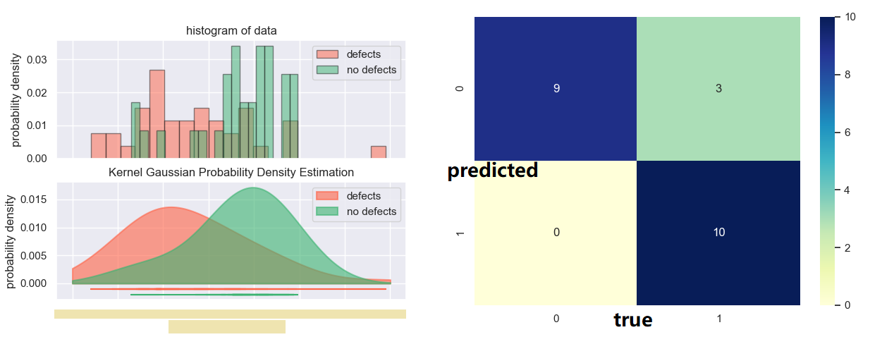
 Based on the original methods that I developed and therefore the machine learning model trained, the accuracy of the model reaches 86.3%, with p values for both method coefficient below 0.1.